Integer Linear Programming Problems: Complete guide

The formulation of integer linear programming problems is often encountered in business situations where resources are limited and demand for them is sufficiently high.
It is a mathematical programming technique used to solve problems related to the optimal allocation of scarce resources among activities that compete for their use. Resources can be time, money, or materials, and the constraints are known as constraints.
✅ Components to be used in the integer Linear Programming Problems
These models have 3 fundamental components to identify, which we develop below:
Decision variables: Variables representing the options under the control of the decision-maker.
Objective function: An expression in the linear programming model that mathematically states what is to be maximized (e.g., profits or present value) or minimized (e.g., costs or waste).
Constraints: Limitations that restrict the permissible options for decision variables.
The effective formulation of a linear programming problem involves the identification and understanding of its three essential components.
First, decision variables are the key elements representing the available options under the control of the decision-maker. These variables, when manipulated, directly influence the model’s outcomes.
On the other hand, the objective function constitutes a fundamental mathematical expression in the framework of linear programming. This expression clearly states what is sought to be maximized (such as profits or present value) or minimized (such as costs or waste), providing a quantifiable goal for decision-making.
Furthermore, constraints play a crucial role in problem formulation. These limitations outline the permissible options for decision variables, adding a level of realism to the model.
Constraints can arise from various sources, such as limited resources or specific regulations. The ability to efficiently balance these constraints while working towards optimizing the objective function is essential for the success of linear programming.
In summary, by understanding and properly applying the components of decision variables, objective function, and constraints, a solid foundation is established for the effective formulation and resolution of linear programming problems, enabling informed and strategic decision-making in various business situations.

✅ Requirements and Assumptions for integer Linear Programming Problems
The formulation of a linear programming problem requires careful attention to the fundamental requirements and assumptions that support it. First and foremost, the model must be designed to maximize or minimize a critical variable identified as the objective function. This clear and quantifiable focus establishes the central purpose of the model, providing direction for decision-making. Resource limitation is another key requirement, as scarcity and resource constraints form the basis of many problems addressed through linear programming.
Linearity emerges as an essential principle in this context, where both the objective function and constraints are expressed as linear functions. This characteristic allows for a more manageable and efficient mathematical representation. Certainty in parameter values is an underlying assumption, as linear programming assumes that these are known and constant during problem solving.
The divisibility of products and resources is a crucial aspect, allowing variables to take non-integer values. This flexibility is essential for addressing situations where the quantity of products or resources is not limited to integer values. Finally, homogeneity, which implies the absence of economies of scale, is an assumption that contributes to maintaining simplicity and clarity in problem formulation.
Taking into account the requirements and assumptions of maximization/minimization, resource limitation, linearity, certainty, divisibility, and homogeneity establishes a robust framework for addressing complex problems through linear programming. This provides a structured basis for strategic decision-making in business and operational environments.
In summary:
We can say that to develop a model of these characteristics, it is necessary for it to have the following characteristics:
- They must seek to maximize or minimize a critical variable (which we will call the objective function).
- Resources are limited.
- Linearity: the objective function and constraints are expressed as linear functions.
- Certainty: parameter values are known and constant.
- Divisibility of products and resources, implying that variables can take non-integer values.
- Homogeneity: there are no economies of scale.
✅ Example Case of Formulating integer Linear Programming Problems
Let’s suppose you are in charge of organizing a work team for the manufacturing of a new product. For this, you have a staff of 30 professionals and 20 technicians from which you can take labor. According to the labor agreement, it is necessary to have an equal or greater number of technicians than professionals and the number of technicians should not exceed twice the number of professionals.
In the tool shed, you have 50 tool kits available to manufacture this product. It is known that each professional takes one toolkit from the shed, while each technician takes two.
The profit contributed per day by each member is estimated at: $150 per professional and $120 per technician.
The 3 steps for setting up the model
Steps for Formulating Linear Programming Models
To begin formulating the model, let’s go back to the 3 fundamental steps, which are: define decision variables, identify case constraints, and define the objective function.
Step 1: Identify Decision Variables
Which variables are under our control?
In this case, we could identify 2 variables:
- X = Number of professionals
- Y = Number of technicians
Step 2: Identify Constraints
Once the decision variables are defined, the next step is to define constraints based on them. For this problem, the constraints would be:
50 tool kits: professionals use 1 and technicians use 2. ➡️ X + 2Y <= 50
Number of technicians does not exceed twice the number of professionals. ➡️ Y <= 2X
Labor agreement: equal or greater number of technicians than professionals. ➡️ X <= Y
Available personnel quantity: ➡️ X <= 30 ➡️ Y <= 20
Non-negativity: ➡️ X and Y > 0
Step 3: Identify Objective Function
The profit contributed per day by each member is estimated at: $150 per professional and $120 per technician. We can then define the objective function as the following maximization (maximized due to the coefficients being profits):
Max(Z) = 150 * X + 120 * Y
✅ Graphical Solution of the integer Linear Programming Problems
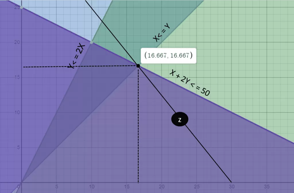
To find the optimal solution, we can do it using a graphing tool like Desmos. We will find the optimal solution graphically at one of the vertices of the feasible region. Feasible region is where all its points are possible solutions, and the vertices represent possible optimal solutions.
The way to do this is by giving various values to the objective function (i.e., to Z) until we find the value that touches the feasible region at its furthest point from the origin.
The optimal solution for this exercise is the point furthest from the origin that intersects the feasible region. In our case, this point is the vertex (16.667, 16.667) as shown in the image.
Animated Resolution in DESMOS
“If you cannot visualize the resolution in DESMOS, access it by clicking here.
✅ Mathematical Resolution of the Linear Programming Model
Next, we show the mathematical resolution. To do this, we must first focus on the graph. As we can see, the optimal solution is composed of the constraints X + 2Y <= 50 and X <= Y. Therefore, the optimal solution is the point formed by the intersection of these two lines. To calculate the intersection point of these two lines, we simply need to set up a system of 2 equations with two unknowns (x and y). Below is the mathematical resolution.
X<=Y ➡️ X = Y
Next, we replace the previous equation into the other constraint, X + 2Y <= 50, and thus leave the following equation:
X + 2*(X) = 50
Then, the solution is:
X= 16,667
y= 16,667
✅ What Decision to Make? From Theory to Practice in solving integer Linear Programming Problems
Given the previous exercise, what decision should the company make when hiring?
In reality, since resources are people, we will have to take INTEGER values for X and Y.
So, if we round (up or down), we could evaluate the following 4 points:
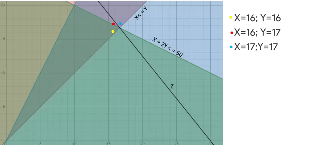
X=16; Y=16 ✔️
X=16; Y=17 ✔️
X=17; Y=17 ✖️ This option is NOT feasible because it does not meet the constraint X+2Y<=50, since 17+17*2=51
X=17; Y=16 ✖️ This option is not feasible because it does not meet the constraint X<=Y since 17 is not less than 16
Having said that, we can see that the decision to be made is between points 1 and 2. If we analyze it graphically in the following image, we see that with the slope of Z, the furthest point from the origin is X=16; Y=17.
Although we have already checked it graphically, if we do it mathematically by replacing these two sets of points in the objective function, we will see that option 2 has a higher Profit:
- X=16; Y=16 ➡️ Z=15016+12016 =$4320
- X=16; Y=17 ➡️ Z=15016+12017 =$4440
Since the values of x and y must be integers and also, since the number of technicians must be greater than or equal to the number of professionals, x=16; y=17 is the optimal solution that maximizes profits at $4440.
Although the mathematical solution is x=16.66 ; y= 16.66, and with a profit of $4500, we see that this is not feasible due to the need for the solution to be integers. We see that the difference between the mathematical model and the implemented solution is +$60.