Linear Programming: minimize costs and maximizes profits.

Linear programming is an operations management tool used in business situations where resources are limited and demand for them is high.

In other words, it is a mathematical programming technique used to solve problems related to the optimal allocation of scarce resources among activities that compete for their use. The resources referred to can be time, money, or materials, and the limitations are known as constraints of the production system. For these types of problems, we aim to minimize costs/expenses and maximize profits.

✅ Where Does Linear Programming Come From?

Linear programming, a cornerstone in the field of operations research, has evolved significantly from its early concepts to become an indispensable tool in business and governmental decision-making. Its historical development has been a fascinating narrative, marked by key contributions from visionary mathematicians and practical applications that have transformed the efficient management of resources.

In the mid-20th century, figures such as George B. Dantzig and Leonid Kantorovich laid the theoretical foundations of linear programming. The formulation of mathematical models for the optimal allocation of resources in situations with linear constraints led to revolutionary algorithms, such as the Simplex Method developed by Dantzig in the 1940s. This method provided an effective solution to linear optimization problems, opening doors to practical applications in supply chain management, production, and logistics.

The 1970s witnessed the rise of linear programming in strategic planning and corporate decision-making. The development of specialized software allowed for the efficient resolution of more complex problems, solidifying the position of linear programming as an essential tool in operations research.

In the 21st century, linear programming has further evolved with the integration of advanced techniques such as convex optimization and nonlinear programming. Its application extends to diverse fields such as engineering, economics, health, and artificial intelligence, demonstrating its versatility and continued relevance in an increasingly complex and globalized world. In summary, linear programming has not only left an indelible mark on the history of operations research but also remains a guiding light for efficiency and informed decision-making today.

✅ Introduction to Linear Programming

We’ve already provided a brief theoretical introduction to what linear programming entails, but when we delve deeper into practical industry terms, we should ask ourselves: when is it worthwhile to optimize something?

Let’s consider a scenario with an example. Suppose you are tasked with the role of operations manager at a medical supplies factory. It’s known that the factory produces a single product (only 1 SKU) with a high gross profit margin. Additionally, it’s known to have the following characteristics:

• It has infinite availability of raw materials.
• It has infinite available capacity.
• It has infinite demand.

How much would you manufacture?

One might think that with infinite demand and availability of resources, we should manufacture as much as possible.

However, what if suddenly the availability of raw material becomes finite? In this new scenario, how much would you manufacture?

New scenario:

• It has finite availability of raw materials.
• It has infinite available capacity.
• It has infinite demand.

Clearly, in this case, with infinite demand, we would try to manufacture as much as possible. The difference from the previous case is that now, with a limitation on access to raw materials (because it’s no longer infinite and is now finite), that maximum potential will be restricted by the availability of raw materials. In this sense, we can say that raw material becomes the scarce resource in our model, as available capacity and demand remain infinite.

Now, if we also introduce another limitation on demand, how much would you manufacture?

New Scenario:

• It has finite availability of raw materials.
• It has infinite available capacity.
• It has finite demand.

Following the logic of the previous case, we should begin by analyzing what has ceased to be infinite and has become finite. In this case, it’s the availability of raw materials and demand. The question of how much to manufacture now begins to incorporate the logic of linear programming where the constraints of a model start to compete. In this case, the constraint of raw material and the constraint of demand converge to seek an optimum. The answer to how much we should manufacture is determined by the quantity that maximizes revenue based on maximum demand and the quantity of raw materials available.

The above is just an example of the development of simple linear programming problems. They can become more complex by adding more variables, such as a variety of products. Instead of producing one product model as in the previous case, there could be many more. Additionally, the model could become even more complex if we see that all these product designs competing to be manufactured have different profit margins and different demand volumes. As we add data to the model, all these factors culminate in a great difficulty in efficiently managing resources, which without the knowledge of linear programming, would be impossible to resolve.

✅ Linear Programming as an Optimization Tool in Supply Chain Management

In the fast-paced world of supply chain management, tackling complex problems may seem daunting. But how do we solve these problems? This is where mathematical programming comes into play, a powerful family of optimization methods that has become the shining knight in armor for logistics professionals.

Family of Optimization Methods
Mathematical programming encompasses various techniques and methodologies, with three standing out in particular:

1. Linear Programming (LP): Ideal for maximizing or minimizing linear functions under certain constraints.
2. Integer Programming (IP): Introduces the constraint that variables must be integers, adding an additional level of complexity.
3. Mixed-Integer Linear Programming (MILP): Combines elements of linear and integer programming to address more challenging and realistic problems.

Why Use Mathematical Programming?

Essential Approach in Supply Chains
The primary reason is that mathematical programming has established itself as the most widely used approach in supply chain management. From network design to production planning, selection of logistics providers, inventory allocation, and port/terminal operations planning, this methodology offers optimal and efficient solutions.

Unmatched Accessibility
Don’t worry about complexity. Mathematical programming is at your fingertips. Most supply chain management software or tools incorporate this methodology, facilitating its implementation in various areas of your company.

From spreadsheets to other management tools, mathematical programming has been seamlessly integrated into the technological solutions you use daily.

Identification of the “Best” Solution
When faced with constraints and aiming to find the optimal solution, mathematical programming emerges as the best way to identify that “best” solution. It allows you to optimize operational processes and resources, ensuring that your decisions are backed by a quantitative and precise approach.

In summary, by adopting mathematical programming in supply chain management, you are investing in efficiency, optimization, and informed decision-making. Don’t let problems overwhelm you; let equations guide you to effective solutions!

✅ Components of Linear Programming Models

There are three main components in linear programming models:

1. Decision Variables: These variables represent the options that are under the control of the decision-maker.
2. Objective Function: An expression in the linear programming model that mathematically states what is to be maximized (e.g., profits or net present value) or minimized (e.g., costs or waste).
3. Constraints: Limitations that restrict the permissible options for the decision variables.

✅ Applications of Linear Programming in Businesses and Industries

Linear programming finds crucial applications in businesses and industries for resource optimization. From supply chain management to efficient allocation of financial resources, linear programming helps maximize profits and minimize costs. Sectors such as logistics, manufacturing, finance, and strategic planning use this tool to make informed and efficient decisions that contribute to business performance and profitability.

Below are some examples of how linear programming is applied in businesses and their objectives.

Examples of Linear Programming in Industries

1. Shift Planning: It can also be applied in services. In this case, it aims to find the assignment of workers per shift to produce at minimum cost under variable demand.
2. Process Control: From a quality management perspective, linear programming aims to minimize the amount of waste material generated in the cutting of steel, leather, or fabric from a roll or sheet of stored material.
3. Inventory Control: Determining the optimal combination of products stored in a warehouse.
4. Distribution: Finding optimal allocations for shipments from factories to distribution centers.
5. Plant Location Study: Determining the optimal location of a plant by evaluating shipping costs between alternative locations, based on existing supply and demand sources.
6. Optimal Product Routing: Determining the optimal route of a product that needs to be sequentially processed in several machine centers, with each machine having its own cost and production characteristics.
7. Vehicle Scheduling: Assigning vehicles to products and determining the number of trips, depending on the size of the vehicle, its availability, and demand constraints.

These applications demonstrate how linear programming is a versatile tool that can be applied across various industries to improve efficiency, reduce costs, and enhance overall performance.

✅ Example Case of Linear Programming Applied to Production Mix Optimization

This case involves a construction company that manufactures high-quality enclosures, including glass windows and doors. Currently, it operates with 3 production plants where Plant 1 produces aluminum frames, Plant 2 produces wooden frames, and Plant 3 produces the glass and assembles the products.

The company decided to manufacture two new products: an 8-foot glass door with an aluminum frame (let’s call it “Product 1”) and a 4×6-foot window with a wooden frame (let’s call it “Product 2”). Each product is manufactured in batches of 20 units, and the production mix is defined in batches per week.

The production manager of this company is a highly committed industrial engineer to the efficient use of resources, so he wants to determine the production mix that maximizes profit.

To begin the analysis, we will create a general process flowchart to understand how the plants and warehouses interact with demand.

Formulation of the Model for this Problem

As explained in this article on linear programming model formulation, for any linear programming problem, it’s crucial to define three fundamental points: decision variables, constraints, and the objective function.

Definition of Decision Variables

To define the decision variables (DV), it is advisable to consider those aspects that are under our control and over which we can influence. In this case, we define the decision variables as follows:

X = # of batches of Product 1 to produce per week

Y = # of batches of Product 2 to produce per week

Identification of Constraints

The second step is to identify the constraints of our model and then express them in terms of the decision variables. Typically, constraints are associated with resources, demand, and other contextual variables. For this example, we can identify the following constraints:

Availability of time for each plant, where:

X <= 4 (Plant 1)

Y<=12 (Plant 2)

3x+2y<=18 (Plant 3)

No-Negativity:

x>=0; y>=0

Definition of the Objective Function (Z Function)

Finally, we must define the objective function. This milestone essentially depends on what we are seeking (whether to minimize costs, minimize the use of a resource, maximize profits, etc.). It is important to note that at this point, problems will always involve maximizing or minimizing some function. For this case, as we are seeking the ideal production mix to maximize profit, we can define our objective function as:

Maximize Z = 3X + 5Y

Where 3 and 5 are the selling values of each product expressed in K$.

Having formulated the problem, we will proceed to solve it by determining the combination of X and Y (quantity to manufacture of doors and windows) that maximizes Z, subject to the availability and non-negativity constraints.

How to Solve this Problem Graphically?

To solve the problem, we will make a two-dimensional graphical representation where each axis represents the decision variables X and Y. We will plot the lines of the constraints and the isoprofit line (Z) on these axes. If you want to learn more about how to graph linear programming models, we recommend reading this article on Graphical Linear Programming.

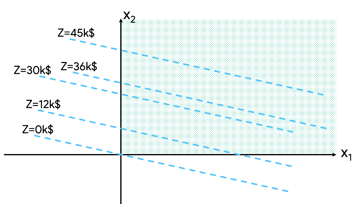
First of all, and by way of example, we will graph different values of Z. In the image below, we can see that the slope of the line arises from the profits per batch. Each line shows the production combination that yields that profit.

Analyzing the objective function

For example, if we adjust the coefficients of the objective function Z (i.e., the revenues obtained for each product), the slopes of the isoprofit lines would be different. Let’s suppose the new coefficients are $10 for product 1 and $6 for product 2. Then, the isoprofit lines would have the following slopes:

• For a profit of $12 (with the previous coefficients), the slopes would be:
  • X = 0 and Y = 2.4
  • X = 4 and Y = 0
  • X = 3.5 and Y = 1
• If we change the coefficients to $10 for product 1 and $6 for product 2, the new slopes would be different, implying different production combinations to achieve the same profit of $12.

This flexibility in the coefficients of the objective function is an important feature of linear programming models, as it allows us to analyze how optimal solutions change with changes in the problem parameters.

Similarly to how we graphed the objective function, let’s graph the constraints of the model outlined earlier. As you can see, the constraints are lines that intersect each other at certain points. The area defined by these lines (shaded in the image) is called the feasible region and is composed of all possible solutions to this linear programming problem.

Finding the Optimal Solution Graphically

When the objective is to maximize and the coefficients are positive, profit increases upwards and to the right (X and Y increase). Therefore, what we need to do is move the line of the Z function in that direction until we can detect the last point it touches in the feasible region.

As we can see in the graphical resolution, the optimal production mix for this model will be 2 units of Product 1 and 6 units of Product 2, with a total profit of $36,000.

Finding the Optimal Solution Mathematically

For this case, we can solve the mathematical problem in two ways. The first is by equating the lines that form the optimal point. By doing this, we will form a system with 2 equations and 2 unknowns. Then, we solve for the values of X and Y that make up the solution.

We can also operate mathematically for each vertex of the feasible region. By obtaining the value of each vertex, we can determine which one is the greatest, i.e., the optimum. This is useful, for example, when two vertices are very close to each other and it is difficult to graphically detect which one is optimal.

The disadvantage of this mathematical method is that it only works for 2 decision variables. When there are more variables, it is recommended to use software such as Excel Solver. In this link, I share an article that shows how to solve the previous exercise using Excel Solver.

✅ Conclusions and Key Points

We can define a procedure for representing this type of problems taking into consideration:

• The number of decision variables determines the dimensionality of the problem space.
• Problems with 2 variables can be represented in a 2-D graph.
• Choose one axis for each variable.
• Constraints determine the set of feasible solutions.
• Each inequality determines a feasible half-plane.
• The feasible region is the intersection of feasible half-planes.
• To graph a constraint, choose two points that satisfy it and draw the line passing through both.
• The feasible half-plane is the one that satisfies the corresponding inequality.
• Choose an arbitrary objective function and draw an iso-profit line by choosing two arbitrary points.
• Find the direction of improvement of the objective function (OF); and locate candidates for optimal vertices.
• Calculate the solution corresponding to each candidate vertex by solving the system of equations of the active constraints at that point.
• Compare objective function values by substituting the coordinates of the candidate solution into the objective function.
• An optimal solution is always found at a vertex.
• Each inequality determines a feasible half-plane.
• The feasible region is the intersection of feasible half-planes.
• To graph a constraint, choose two points that satisfy it and draw the line passing through both.
• The feasible half-plane is the one that satisfies the corresponding inequality.